Portrayed below is a complete and self-contained NEC model of one popular form of the end-fed half-wave dipole antenna. Applying a feed to any antenna in NEC or any electromagnetic simulation software is about a simple a task as can be conceived by placing a “source” of near infinitesimal size inline with a dipole element. Coax? No worries. Impedance? Use a current source. Examples and discussions exist here, here, here, and here. While perfectly fine for various studies, this leaves the trickiest part out of the equation… namely how to change a 50 ohm feed impedance to that appropriate to feed the high impedance end of a half-wave dipole. This study includes the physical model of just such a step-up transformer providing a way to use a 50 ohm source.
Electromagnetic simulation tools
I have access to a wide variety of electromagnetic simulation tools. At opposite ends of the software landscape we have…
FDTD – Finite-Difference Time-Domain method: Actually calculates Maxwell’s equations in time step offering movie like views of the progression of both electric and magnetic fields. Very slow, often high cost software, but very complete and very cool.
NEC – Numerical Electromagnetics Code method: Uses Method of Moments technique to calculate steady state currents of each wire segment. Relatively fast, often low cost or free software and offers an easy entry into antenna simulation.
Since NEC is available to so many, it got the nod for this project. So now what front end to use.
EZNEC or 4nec2
Of the numerous “front ends” available to run NEC, EZNEC and 4nec2 seem to be at the top of the stack.
The recent versions of EZNEC include a transformer emulation capability that might be of interest to end-fed experiments. 4nec2 pretty much relies on whatever the underlying NEC can provide. It truly is a front end to the command-line NEC executable programs. This is actually an advantage for 4nec2 since improved or optimized NEC executables instantly upgrade its speed and computational power. Such is the case with the availability of NEC-MP that recompiles NEC into a truly multi-threaded program. This takes advantage of machines with spare threads and speeds up NEC computations enormously.
Another advantage of 4nec2 is the ability to parameterize dimensional and RLC values to perform optimization and evolution techniques to play “what if” with great ease. One disadvantage of 4nec2… it’s buggy as hell and great care must be applied to watch out for issues. Regardless, 4nec2 gets the nod for this effort.
How to model the transformer in NEC
Simulation packages such as EZNEC offer special transformer simulation. Sounds very handy and I look forward to learning how this works someday. However, I wanted to study the behavior of the entire system including the winding of the step-up transformer rather than rely on an idealized version of same.
Years ago I took an antenna class from Dr. Stephen Best who was kind enough to field questions after the class. At that time I was designing an improvement to the Super J antenna to replace the Franklin stub with a coil. I knew much could be accomplished in NEC using an inductance inline, but asked him for tips regardless. He said “Why not just simulate the inductor as wires along with the rest of the model?” I did and it worked well. Of particular significance is the ability of NEC to provide a better realization of a coil than any idealized and perfect inductor.
Time to make the model.
NEC model of the end-fed half-wave dipole antenna
Taking the lessons from the Super J and Dr. Best, I set about to simply design a helical step-up transformer at the end of a half-wave antenna element. It took some trial and error with the tools available in 4nec2, but wound up with this design in figure 1.
Figure 1 – The end-fed half-wave dipole antenna with magnified view of transformer.
Features include:
Approximately one half wavelength of straight wire from the antenna top to the top of the transformer winding.
20:3 step-up transformer in the autotransformer configuration. Various ratios were tried until discovering 20:3 produces close to 50 ohms (for this particular situation).
The transformer configuration produces an inductive component at the 3rd tap wire. A reactance, Xs, is in series between the source and the primary winding to provide the means to compensate for this.
This is a core-less air transformer (or “air core” if you like) just in case that isn’t obvious.
That series reactance is most often a capacitor in series. It’s what one finds in end-fed VHF and UHF antenna systems from Diamond Antenna and others. One example is the NR770HBNMO end-fed dual band mobile antenna and companion K515S Luggage Rack Mount groundless mount. Numerous web sites reveal the coil and series capacitor of these antennas.
No “extra” counterpoise or other conductors required
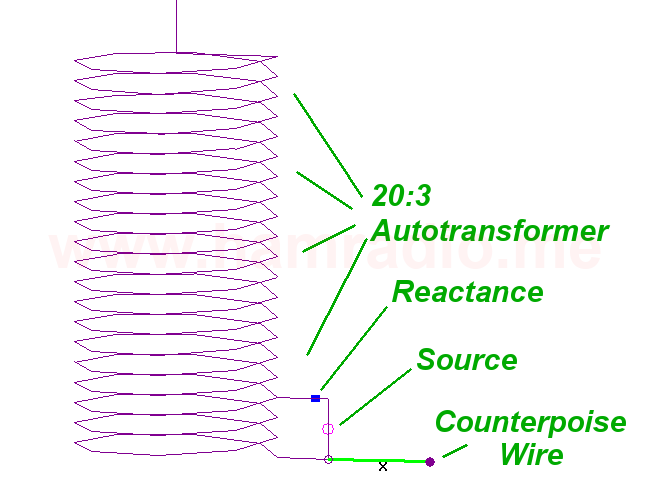
Figure 2 – The transformer converting 50 ohms to the thousands one needs to drive the current node of a dipole.
Danger, Danger, Danger!!!
I probably am using the term counterpoise incorrectly, but there is so much variation in its use, oh well. Owen Duffy suggests avoiding the term and I cannot disagree, but for the sake of this discussion I’m simply referring to any additional conductor beyond that of the EFHW antenna system (whip, coil, reactance and source). Cool? Alrighty then let’s move along.
Figure 2 gives a bit more detail highlighting the location of the source and reminding us eventually something will connect to the feed point and provide a bit of counterpoise. However one point for this particular effort was to prove to myself this can work without need of a purpose-built counterpoise system or other conductors. Hence the wire in light green does not actually exist in the simulations for this article.
Okay yeah the little bit of wire coming out from the transformer to meet the source and reactance do provide a little bit of counterpoise, but to what effect. Hint, the effect of the extra wire will be covered in depth in a forthcoming article.
The impedance seen by the source
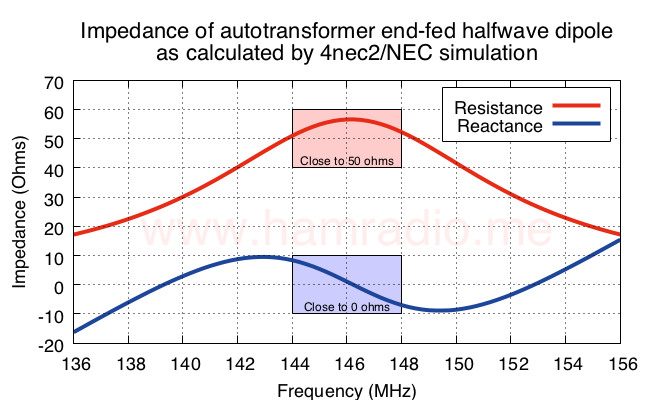
Figure 3 – Final impedance after insertion of series capacitor to offset inductive reactance of the end-fed half-wave dipole antenna.
Figure 3 shows the resistance and reactance as seen by the source as configured in figure 1. Pretty darn nice if you ask me. The resistance swings quite close to 50 ohms thanks to the “turns ratio” of the autotransformer. The reactance hovers near zero thanks to the compensating series capacitance.
Let’s explore more about that series compensating capacitance.
Inductive antenna without a series capacitor
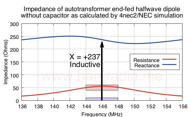
Figure 4 – Resulting inductive feed point impedance with no series capacitance.
The combination of the transformer with the end-fed dipole results in a positive reactance. This suggests an inductive reactance. The resistance (real) component of the impedance is right where we want it near 50 ohms. This reveals we only need to compensate for the reactive component. A series capacitance, Xs in figure 1, is the easiest approach for this example.
Calculating the value for Xs
Knowing we need a Capacitive Reactance, we can review the definition to take the next steps. Compensating for +237 ohms merely requires an offsetting -237 ohms from the capacitive reactance. We head to the formulas where Xc stands for Xs.
We swap Xc and C and make Xc = 237 ohms and f = 146,000,000. Solving for C results in a capacitor of value 4.59 pF to provide the -237 ohm reactance to compensate for the antenna/transformer inductive reactance.
The effect of series capacitance on resistance
Let’s see what happens to the real value resistance of the antenna system as we dial in the correct capacitance.
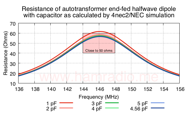
Figure 5 – How the series capacitor affects the feed point resistance.
As one expects, the real value of the inductance changes little with the varying series capacitance. It is most perturbed with the 1 pF value, but settles in as capacitance gets well beyond the “mere open gap” values. More about 4.56 pF in a moment.
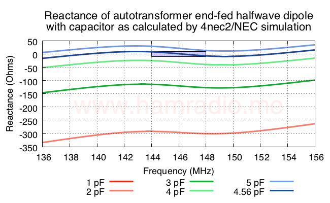
The effect of series capacitance on reactance
Figure 6 – How the series capacitor affects the feed point reactance.
The final reactance presented to the source varies wildly as capacitance increases from 1 pF to our goal. 5 pF overshoots a bit as we expect. Simulation optimizations reveal 4.56 pF brought the net reactance to zero ohms. This is very close to our predicted value… pretty much a bulls eye. There are some parasitic capacitances in play as well, but this result offers good agreement of theory and simulation.
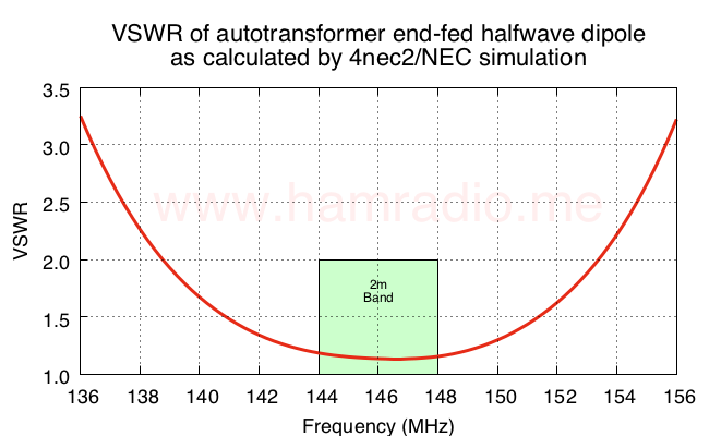
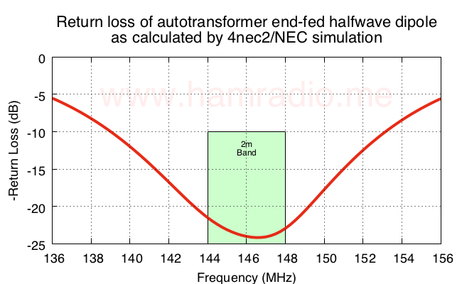
Resulting antenna match
The results speak for themselves.
Figure 7 – VSWR of end-fed half-wave dipole antenna.Figure 8 – Return loss of end-fed half-wave dipole antenna.
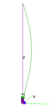
Resulting antenna current
Figure 9 – The resulting current distribution of the end-fed half-wave dipole antenna.
Nice… boring… dipole…
fed at its end…
with no significant counterpoise system or other extraneous conductors…
or “other half” of the antenna to <cough>push against</cough>.
Hallelujah.
For those that might be interested, the peak value of current in the middle of the dipole confirms the 100 watts form the source winds up on the element. This assumes the mid point impedance is about 70 ohms. Thus the energy from the source finds its way to the dipole for radiating.
Resulting gain
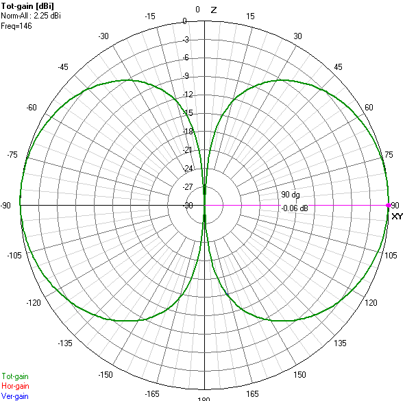
The 0.967 AGT (-0.15 dB) from the NEC4 simulation indicates enough deviation to account for the overly ambitious 2.25 dBi value of the gain shown in figure 10.
Figure 10 – EFHW_Antenna Gain in the E-plane
The compensated gain comes to about 2.1 dBi, close to a perfect dipole’s 2.15 dBi gain. Further tweaking of the model can likely improve this, but that’s beyond the larger point of this article.
Conclusion
Here is the 4nec2 model file with .txt appended (you’ll need to remove .txt) for you to play with.
The goal for a wire model of an end-fed half-wave dipole antenna with no special simulator tricks (like EZNEC’s transformer function) is achieved.
The impedance conversion function of the wire helix autotransformer is no problem for NEC4 although annoying trial and error were required to find the 20:3 ratio that worked well in this mathematical world of simulation.
A bunch of wire and a series capacitance can yield an EFHW antenna.
Yes this is a closed system of perfect conductors so of course the energy moves through the model well, but the success of keeping return loss managed suggests this is a viable antenna topology. As a result, antenna manufacturers abound with models pretty much like the above. This shouldn’t be news to antenna professionals. One can hope this information helps offset some of the “other half” and “push against” points seen in the great EFHW debates found on The Zed and other amateur radio watering holes.
14 thoughts on “Simulating the end-fed half-wave (EFHW) dipole antenna”
Very nice article, I have a commercial EFHW antenna for 2M like you have analyzed. An interesting fact is that Dr. Best was my job interviewer and I also learned a lot from him too. He was very supportive of my "weird" antenna designs at Cushcraft Corp. some 20+ years ago. Keep up the great work…73 Danny Horvat, E73M aka MyAntennas.com
Wow. I am impressed with the well written article, the effort to develop the transformer coil and the handling of the reactance. However, the model is not what I would publicize yet because of the very poor AGT value. Some more work is needed to see what is wrong or even if NEC2 can handle it. Maybe take a look at what is generating the 135 MHz secondary resonance.
Points well taken. I found 0.967 AGT with NEC4. I guess I should have a look at NEC2 results as well. I've never been too sure how far off AGT can be before trouble begins. What I really want to do is actually make the thing, but I'm busy with another EFHW experiment at the moment. If you find a design tweak that yields better results with NEC2 please consider sharing.
What is that little green horizontal piece and why do we need it?
I can see that the little green piece will not support an average 'standing' current as seen in the 1/2 wave section.
Being very short, any current should drop to zero at the end.
I am curious about the potential. How does it look across the coil (both ends and tap).
I am also and mostly curious as to how charge is distributed as a function of time, as it must be conserved.
Thanks, -bob
The little green wire reminds is we always have something attached to the feedpoint, but isn't a hard requirement to get the assembly without wire to resonate. Figure 2 is really about this article… https://www.hamradio.me/antennas/of-end-feds-and-…
The potential, with respect to the middle of the dipole section, is quite high. Wherever there is potential, there is charge.
What is that little green horizontal piece and why do we need it?
What does the little "x" near themiddle of the horizontal piece represent.
I'm not sure my whole question made the post.
Mostly curious about charge distribution as a function of time.
I am not familiar with the modeling software and table entries but I understand the structure.
The coil wire has a resistance as does the wire making the ~ 1 m section. If I read correctly you've used a 1.25 mm diameter wire for both.
I can not see any resistance values in the table.
A 1.25 mm copper wire has a resistance at 147 MHz of ~ 0.8 ohms per meter. Aluminum will be ~1 ohm per meter.
What value did you use in your model?
How does the model look (Q and efficiency) when you use a 0.8 ohm per meter value for the wire.
"If I read correctly you've used a 1.25 mm diameter wire for both." 1.27 mm
"I can not see any resistance values in the table." It is currently PEC.
"What value did you use in your model?" 0 ohms
"How does the model look (Q and efficiency) when you use a 0.8 ohm per meter value for the wire." Good question. I set the conductors to stainless, aluminum and copper. Efficiency was lowest for stainless steel at 92%. Everything else was better. Bandwidth did change a bit, but nothing significant.
I admire the effort that went into producing that paper.
Downloading and running your .nec file produced a question, though: Doesn't the short vertical conductor leading away from Terminal #2 as shown in the graphic linked below constitute the second conductor needed for the "EFHW" to radiate, even as short as it is? https://i.postimg.cc/rFdkggP6/JSH-2m-EFHW-Detail….
Yes, absolutely. The "end-fed" moniker does seem to imply a single terminal source, but all power sources are certainly two terminal devices. It's a game of semantics isn't it? In my mind "end-fed" refers to the radiator feed, but I could be wrong. The larger question is if point #2 requires "extra" treatment of ground, lengthly counterpoise or other ideas to get radiation from the dipole radiator. This simulation suggests no as does my experiment with a 10 MHz dipole here… https://www.hamradio.me/antennas/electrically-iso…
The problem, of course, is we can never really get a power source infinitely small so even its body will be a bit of electrical "mass" (or counterpoise if you like) to push against, but the data seems to be suggesting it doesn't have to be electrically large. Put another way, there's nothing about the EFHW that is fighting our ability to energize it so long as we handle the impedance transformation… and that's the larger point here.
RE: " In my mind "end-fed" refers to the radiator feed, …"
But the conductor attached to Terminal #2 in my graphic forms part of the "radiator" as much as the conductor attached to Terminal #1, doesn't it? Just a lot shorter.
IMO, that path attached to Terminal #2 of the source is not correctly thought of, or described as a counterpoise — rather it is one side of a (very) off-center-fed dipole.
"IMO, that path attached to Terminal #2 of the source is not correctly thought of, or described as a counterpoise — rather it is one side of a (very) off-center-fed dipole."
I thought this as well… especially given the existence of dipoles fed somewhere between mid and end: offset fed. My simulations and the measurement of the case with extra 0.05 wave wire shown here… https://www.hamradio.me/antennas/adding-0-05-wave…
…seem to suggest the extra wire, while certainly pulling a bit of current, isn't part of the grander sinusoidal current distribution of the primary dipole element. Thus the resonant frequency of the overall system changes little. It's as if the feed point is a demarcation line between independent antennas, each managing their own destiny whereby they draw current if they present a matching HiZ to the feed.
I shared your opinion originally, but the evidence just isn't supporting it.
It is Fuchs antenna from the 1930's.
Comic to simulate and exactly analyze circuits that resonate with the environment. After the next rain you can start tuning over again.


Very nice article, I have a commercial EFHW antenna for 2M like you have analyzed. An interesting fact is that Dr. Best was my job interviewer and I also learned a lot from him too. He was very supportive of my "weird" antenna designs at Cushcraft Corp. some 20+ years ago. Keep up the great work…73 Danny Horvat, E73M aka MyAntennas.com
Wow. I am impressed with the well written article, the effort to develop the transformer coil and the handling of the reactance. However, the model is not what I would publicize yet because of the very poor AGT value. Some more work is needed to see what is wrong or even if NEC2 can handle it. Maybe take a look at what is generating the 135 MHz secondary resonance.
Points well taken. I found 0.967 AGT with NEC4. I guess I should have a look at NEC2 results as well. I've never been too sure how far off AGT can be before trouble begins. What I really want to do is actually make the thing, but I'm busy with another EFHW experiment at the moment. If you find a design tweak that yields better results with NEC2 please consider sharing.
What is that little green horizontal piece and why do we need it?
I can see that the little green piece will not support an average 'standing' current as seen in the 1/2 wave section.
Being very short, any current should drop to zero at the end.
I am curious about the potential. How does it look across the coil (both ends and tap).
I am also and mostly curious as to how charge is distributed as a function of time, as it must be conserved.
Thanks, -bob
The little green wire reminds is we always have something attached to the feedpoint, but isn't a hard requirement to get the assembly without wire to resonate. Figure 2 is really about this article…
https://www.hamradio.me/antennas/of-end-feds-and-…
The potential, with respect to the middle of the dipole section, is quite high. Wherever there is potential, there is charge.
What is that little green horizontal piece and why do we need it?
What does the little "x" near themiddle of the horizontal piece represent.
I'm not sure my whole question made the post.
Mostly curious about charge distribution as a function of time.
The "x" is an axis marking. I probably should have removed it to make the picture prettier.
Thanks.
I am not familiar with the modeling software and table entries but I understand the structure.
The coil wire has a resistance as does the wire making the ~ 1 m section. If I read correctly you've used a 1.25 mm diameter wire for both.
I can not see any resistance values in the table.
A 1.25 mm copper wire has a resistance at 147 MHz of ~ 0.8 ohms per meter. Aluminum will be ~1 ohm per meter.
What value did you use in your model?
How does the model look (Q and efficiency) when you use a 0.8 ohm per meter value for the wire.
-Bob
"If I read correctly you've used a 1.25 mm diameter wire for both." 1.27 mm
"I can not see any resistance values in the table." It is currently PEC.
"What value did you use in your model?" 0 ohms
"How does the model look (Q and efficiency) when you use a 0.8 ohm per meter value for the wire." Good question. I set the conductors to stainless, aluminum and copper. Efficiency was lowest for stainless steel at 92%. Everything else was better. Bandwidth did change a bit, but nothing significant.
I admire the effort that went into producing that paper.
Downloading and running your .nec file produced a question, though: Doesn't the short vertical conductor leading away from Terminal #2 as shown in the graphic linked below constitute the second conductor needed for the "EFHW" to radiate, even as short as it is?
https://i.postimg.cc/rFdkggP6/JSH-2m-EFHW-Detail….
Yes, absolutely. The "end-fed" moniker does seem to imply a single terminal source, but all power sources are certainly two terminal devices. It's a game of semantics isn't it? In my mind "end-fed" refers to the radiator feed, but I could be wrong. The larger question is if point #2 requires "extra" treatment of ground, lengthly counterpoise or other ideas to get radiation from the dipole radiator. This simulation suggests no as does my experiment with a 10 MHz dipole here…
https://www.hamradio.me/antennas/electrically-iso…
The problem, of course, is we can never really get a power source infinitely small so even its body will be a bit of electrical "mass" (or counterpoise if you like) to push against, but the data seems to be suggesting it doesn't have to be electrically large. Put another way, there's nothing about the EFHW that is fighting our ability to energize it so long as we handle the impedance transformation… and that's the larger point here.
RE: " In my mind "end-fed" refers to the radiator feed, …"
But the conductor attached to Terminal #2 in my graphic forms part of the "radiator" as much as the conductor attached to Terminal #1, doesn't it? Just a lot shorter.
IMO, that path attached to Terminal #2 of the source is not correctly thought of, or described as a counterpoise — rather it is one side of a (very) off-center-fed dipole.
"IMO, that path attached to Terminal #2 of the source is not correctly thought of, or described as a counterpoise — rather it is one side of a (very) off-center-fed dipole."
I thought this as well… especially given the existence of dipoles fed somewhere between mid and end: offset fed. My simulations and the measurement of the case with extra 0.05 wave wire shown here…
https://www.hamradio.me/antennas/adding-0-05-wave…
…seem to suggest the extra wire, while certainly pulling a bit of current, isn't part of the grander sinusoidal current distribution of the primary dipole element. Thus the resonant frequency of the overall system changes little. It's as if the feed point is a demarcation line between independent antennas, each managing their own destiny whereby they draw current if they present a matching HiZ to the feed.
I shared your opinion originally, but the evidence just isn't supporting it.
It is Fuchs antenna from the 1930's.
Comic to simulate and exactly analyze circuits that resonate with the environment. After the next rain you can start tuning over again.